Translate

Saturday, January 3, 2015

Why Emperor Penguins are not Endangered by Climate Change


Blinded by Beliefs?: The Straight Poop on Emperor Penguins

Adapted from the chapter The Emperor Penguin Has No Clothes in Landscapes & Cycles: An Environmentalist’s Journey to Climate Skepticism by Jim Steele and initially posted to Watts Up With That and Landscapes And Cycles on July 1, 2014 


Two recent press releases concerning the Emperor Penguin’s fate illustrate contrasting forces that will either advance or suppress trustworthy conservation science. The first study reminds me of Mark Twain’s quip, “Education consists mainly in what we have unlearned.” Embodying that truism is a paper by lead author Dr. Michelle LaRue who reports new advances in reading the Emperor Penguin’s fecal stains on Antarctic sea ice that are visible in satellite pictures. Two years ago the fecal stain method identified several large, hitherto unknown colonies and nearly doubled our estimate of the world’s Emperor Penguins.1,2 That didn’t mean climate change had necessarily increased penguin numbers, but a larger more robust population meant Emperor Penguins were far more resilient to any form of change.
LaRue’s new study advances the science by analyzing the shifting patterns of penguin poop, and her results are prompting some scientists to “unlearn” a key belief that has supported speculation of the Emperors imminent extinction. Believing Emperors are loyal to their breeding locations (philopatry), whenever researchers counted declining penguins at their study site, they assumed the missing penguins had died. However other studies had shown populations could suddenly double, and such observations challenged the notion of philopatry.10 
The only reasonable explanation for unusual rapid population growth was that other penguins had immigrated from elsewhere, and loyalty to a breeding location was a misleading belief. LaRue’s study confirmed those suspicions by identifying the appearance of freshly stained ice in several new locations.  LaRue rightfully said, “If we want to accurately conserve the species, we really need to know the basics. We’ve just learned something unexpected, and we should rethink how we interpret colony fluctuations.”…."That means we need to revisit how we interpret population changes and the causes of those changes."
Of course several alarmist websites have spun this evidence of an ancient behavior into a "new" behavior forced by climate change disruptions.
Although mistaking unanticipated emigration for a local extinction has been the hallmark of several bad global warming studies, some researchers refuse to unlearn mistaken beliefs. In 2009 scientists argued that a missing herd of caribou that once numbered 276,000, had been extirpated by climate change. But the herd was later found in an unexpected location in 2011 just as native peoples had suggested. 
Likewise the co-author of the penguin extinction papers 3,8, Hal Caswell from the Woods Hole Oceanic Institute, mistakenly interpreted polar bear emigration as evidence of death due to climate change to advocate the bears’ imminent extinction as discussed here and here). He was similarly instrumental in modeling the extinction of the “March of the Penguins” Pt. Geologie colony. (Pt. Geologie Emperor Penguins are also known as the Terre Adelie colony or the Dumont d’Urville colony, named after the adjacent French research station known by the locals as DuDu.). Caswell and his co-authors are now doubling-down on their first prophesy of extinction for DuDu’s penguins to promote a more calamitous continent?wide extinction scenario.
The second paper is more distrubing. In a recent interview posted at ScienceDaily, the lead author Jenouvrier summarized their new extinction study saying, "If sea ice declines at the rates projected by the IPCC climate models, and continues to influence Emperor penguins as it did in the second half of the 20th century in Terre Adélie, at least two-thirds of the colonies are projected to have declined by greater than 50 percent from their current size by 2100." "None of the colonies, even the southern-most locations in the Ross Sea, will provide a viable refuge by the end of 21st century." 
But Jenouvrier’s reference to sea ice’s influence on Emperor penguins during “second half of the 20th century in Terre Adélie” is a belief that should have been wisely abandoned. It was originally based on bizarre speculation in a 2001 paper Emperor Penguins And Climate Change,9 speculations that defied well-established biology and contradicted observations. The most obvious contradiction being Antarctic sea ice has not declined as all climate models predicted, but sea ice has now reached record extent. By attaching flipper bands and monitoring how many banded birds returned to DuDu researchers argued the penguins were less able to survive due to climate change. The paper’s authors, Barbraud et al, reported a 50% population drop from 1970 to 1981, and they blamed a prolonged abnormally warm period with reduced northward sea-ice extent. But any correlation with northward sea ice extent was absolutely meaningless.
Indeed the northward extent of sea ice had varied from 400 to 150 kilometers away from the colony, but the Emperor’s breeding success and survival depends solely on access to the open waters within the ice such as “polynya” and “leads.” That open water must be much, much closer. When open water was within 20 to 30 kilometers from the colony, penguins had easier access to food and experienced exceptionally high breeding success. When shifting winds caused open water to form 50 to 70 kilometers away, accessing food became more demanding, and their breeding success plummeted.7 Yet Barbraud et al absurdly argued that a reduction in sea ice extent, for unknown reasons, had lowered the penguin’s survival.9 It was catastrophic climate change speculation based on nothing more than a meaningless statistical coincidence.
Barbraud also argued that the warming of winter air temperatures from -17° to  -11°C in 1981 contributed to the penguins demise, even though penguins would welcome any respite from deadly cold. When the penguins spend most of their lives swimming in +2°C water, there is no reason to believe the rise to -11°C had any deadly consequences. Again it was nothing more than a statistical coincidence. Yet the journal Nature gladly published their nebulous analyses and climate fear, and then Jenouvrier, Caswell and several climate scientists were using that apocryphal study to predict more catastrophic extinctions.
Below is the graph featured by penguin expert Dr. David Ainley on his PenguinScience website showing a purported connection between the penguins’ decline and rising temperatures. His website argues, “The Emperor Penguin colony where the movie “March of the Penguins” was filmed has been shrinking. The colony ( Pt Géologie) is located in northern Antarctica where temperatures have been steadily rising. In recent years, the ice has become too thin, and so it blows away before the chicks are grown. Therefore, fewer and fewer young penguins have been returning to live in this colony. Most Emperor Penguin colonies occur much farther south where temperatures are still very cold. This could change, however, if global warming trends continue.”

March of the Penguin colony temperature trends

Seasonal Temperatures from the British Arctic Survey 
The blue arrow in Figure A. suggesting “steadily rising” temperatures, is a figment of Ainely’s imagination. The actual temperatures for the DuDu research station are seen in Figure B. Ainley and I had been involved in several pleasant and thoughtful email discussions about the decline of DuDu’s Emperors, when I became aware of his Fig. A. I emailed him and asked how he justified such a false representation. He apologized and promised to remove it saying, “My intent with the graph was to refer to the temperature trend, a period when temperature was increasing. Sorry about that.” I have always had great respect for Ainley’s work and from our discussion felt a kindred spirit and dedication to being good environmental stewards. But 2 years have passed and his bogus graph remains as of this writing. Perhaps it will be removed if enough people object to its the gross misrepresentation.
Despite satellite estimates, that more than doubled the population of known Emperor Penguins, the International Union for the Conservation of Nature (IUCN) changed their ranking of Emperors from a species of Least Concern to a Near-Threatened species based on modeling studies blaming the decline of DuDu’s penguins on climate change as presented in Jenouvrier and Caswell’s study
Likewise Ainley’s paper Antarctic Penguin Response To Habitat Change As Earth’s Troposphere Reaches 2°C Above Preindustrial Levels10 had great influence. Ainley believed the DuDu colony had been unable to recover since 1980 because global warming had caused a thinning of the sea ice resulting in a premature loss of sea ice that was drowning chicks. Based on his faith in the models, he warned thinning sea ice would get worse. However there was no evidence for such catastrophic events. So I first contacted Ainley to determine if his “drowning chicks” were based on observation or theoretical beliefs. Ainley confessed his claims were based on a sentence in Barbraud’s paper that stated, “Complete or extensive breeding failures in some years resulted from early break-out of the sea-ice holding up the colony, or from prolonged blizzards during the early chick-rearing period.” The early break-out of the sea-ice holding up the colony was merely a belief consistent with global warming hypotheses.
Mark Twain again provides insight to why bad science so easily goes viral having written, “In religion and politics people's beliefs and convictions are in almost every case gotten at second-hand, and without examination, from authorities who have not themselves examined the questions at issue but have taken them at second-hand from others.” And apparently scientists suffer the same second?hand folly.
Not wanting to succumb to a similar mistake, I emailed Barbraud and asked for the dates during which he had observed an “early break-out of sea-ice holding up the colony”. As it turns out, I was not the only one having difficulty finding that evidence. Dr Barbraud replied, “We are currently doing analyses to investigate the relationships between meteorological factors and breeding success in this species, including dates of sea ice break out, which are relatively difficult to find for the moment!” So why did he ever make the claim of “premature breakouts” in the first place?
Emperor Penguins Huddling Disrupted by Flipper Banding
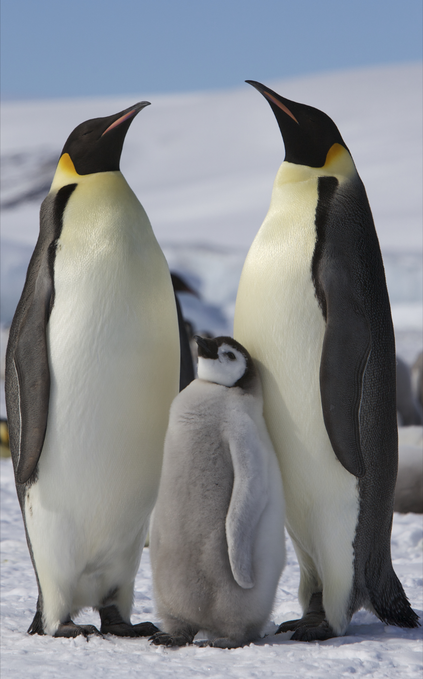
Emperor Penguins Huddle to Conserve LIfe-saving Energy

There is a much more parsimonious explanation for the penguins’ decline. Between 1967 and 1980 researchers from DuDu attached flipper bands to breeding penguins, and that is exactly when the penguins began to desert the colony as seen in Figure A. By the time the much-ballyhooed “warm spike” occurred in the winter of 1981, the colony had already declined by 50%
Several studies have shown that tight flipper bands can increase penguin mortality because flippers can atrophy or swimming efficiency is reduced. Those observations have prompted researchers to argue for another “unlearning” writing, “our understanding of the effects of climate change on marine ecosystems based on flipper-band data should be reconsidered.” 15 However it is unlikely that atrophied flippers from tight bands can fully explain the 50% drop in the Emperor’s abundance. However, interrupting the Emperor’s pair-bonding and vital huddling behavior to attach flipper bands and count birds is a significant disruption that would encourage penguins to seek a more secluded breeding colony.
Placing a band on an Emperor Penguin is no easy task. Male Emperors must conserve energy in order to survive their 4 month winter fast, and tussles with researchers consumed their precious energy. Emperors must also huddle in order to conserve vital warmth (as seen below in the picture from Robertson 2014). But huddling was disrupted whenever researchers “drove” the penguins into files of 2 or 3 individuals in order to systematically read bands or more accurately count the population. “Droving” could also cause the males to drop their eggs that are so precariously balanced on their feet.
When DuDu’s flipper banding finally ended in 1980, coincidentally the Emperors’ “survival rate” immediately rebounded. Survival rates remained high for the next four years despite extreme shifts in weather and sea-ice extent. However, survival rates suddenly plummeted once again in 1985, despite an above-normal pack-ice extent.  Coincidentally, that is when the French began building an airstrip at DuDu, and to that end they dynamited and joined three small islands.


I had argued with Ainley that the only parsimonious explanation for the decline in DuDu’s penguins was that researchers had created such disturbances to their breeding ground, that the Emperors chose to abandon the colony to join others far from such disruptions. Satellite studies such as LaRue’s now support that interpretation as 2 new colonies have been discovered and are the likely home for DuDu refugees.

Yet despite those obvious disruptions, and despite the growing and thickening sea ice, and despite the lack of any warming trend what so ever, the scientific literature is spammed and the public bombarded with more propaganda claiming climate change has put penguins in peril. A peril derived from how they imagined climate change had killed the DuDu penguins in the 1970s.  Robert Bolton wrote, “A belief is not merely an idea the mind possesses; it is an idea that possesses the mind” and catastrophic climate change is tragically possessing too many minds. To repeat LaRue’s advice, if we want to accurately conserve the species, we really need to know the basics.And basically, changing concentrations of CO2 have done absolutely nothing to hurt the Emperor Penguins.


Addendum July 3, 2014
The reason I say I have held Dr. David Ainley in high regard despite our disagreement can be seen in the email I just received, and posted below:

“Hey, Jim, I hope you are doing well!!
Michelle LaRue sent me a link to your blog about the emperor penguin
situation. Sorry to see that I should have deleted that EMPE stuff from
our website back when you and I were discussing it and you were convincing
me that stuff wasn’t adding up. I actually began to write text to revise
the website but kept putting off as other things reared their ugly heads.
Currently, when I do get the revision uploaded — and you’ve shamed me to
do it sooner than later — I’m thinking that it won’t include emperor
penguins at all.
Another reason I have to do this, practical one, is that I’m supposed to
address the Natl Science Teachers annual mtg first week of August (in PA)
and talk to them about penguins and climate change. Been gnashing my
teeth, when thinking about what to say, about the emperor penguin story.
So, now I’ve been kicked in the butt. Thanks!!!
Best regards,
David”

SHARE THIS PAGE:

Literature Cited          
1.Woehler, E.J. (1993) The distribution and abundance of Antarctic and Subantarctic penguins. Scientific Committee on Antarctic Research, Cambridge.
2. Fretwell, P., et al.,, ( 2012) An Emperor Penguin Population Estimate: The First Global, Synoptic Survey of a Species from Space. PLoS ONE.
3. Jenouvrier, S., et al., (2009) Demographic models and IPCC climate projections predict the decline of an emperor penguin population. Proceedings of the National Academy of Sciences, DOI: 10.1073/pnas.0806638106
4. Brahic, C., (2009) Melting ice could push penguins to extinction. NewScientist, http://www.newscientist.com/article/dn16487-melting-ice-could-push-penguins-to-extinction.html. 
5. BBC New, (2009) Emperor penguins face extinction.http://news.bbc.co.uk/2/hi/science/nature/7851276.stm
6. Fraser, A., et al. (2012) East Antarctic Landfast Sea Ice Distribution and Variability, 2000?08. Journal of Climate, vol. 25, p. 1137-1156.
 7. Massom, R., et al. (2009) Fast ice distribution in Adelie land, east Antarctica: interannual variability and implications for Emperor penguins Aptenodytes forsteri. Marine Ecology Progress Series, vol. 374, p. 243-257.
8. Jenouvrier, S., M. Holland, J. Stroeve, M. Serreze, C. Barbraud, H. Wimerskirch and H. Caswell (2014), Climate change and continent-wide declines of the emperor penguin. Nature Climate Change, , doi: NCLIM-13101143-T
9. Barbraud, C., and Weimerskirch, H. (2001) Emperor penguins and climate change. Nature, vol. 411, p.183?186.
10. Kato, A. (2004) Population changes of Adelie and emperor penguins along the Prince Olav Coast and on the Riiser-Larsen Peninsula. Polar Biosci., vol. 17, 117-122.
11. Ainley, D., et al., (2010) Antarctic penguin response to habitat change as Earth’s troposphere reaches 2°C above preindustrial levels. Ecological Monographs, vol. 80, p. 49–66
12. Dugger, K., et al., (2006) Effects of Flipper Bands on Foraging Behavior and Survival of Adélie Penguins (Pygoscelisadeliae). The Auk, vol. 123, p. 858-869
13. Robertson , G. et al (2014) Long-term trends in the population size and breeding success of emperor penguins at the Taylor Glacier colony, Antarctica. Polar Biol (2014) 37:251–259
14. Saraux, C., et al., (2011) Reliability of flipper-banded penguins as indicators of climate change. Nature, 469, 203?206.

Monday, December 29, 2014

Will Greenland Begin Accumulating Ice in 2015 and Beyond?

Based on NOAA’s 2014 Arctic Report Card, the past 2 decades of ice loss in Greenland has slowed dramatically in 2013-2014. In contrast toVelicogna’s (2014) previously published average mass loss of 280 +/-58 gigatons/year using GRACE satellite data, or the maximum loss of 570 gigatons in 2012-2013, there was only an insignificant loss of 6 gigatons from June 2013 to June 2014, or  mere 1% of the previous year’s loss. A loss of 360 gigatons translates into a 1 millimeter rise in sea level, therefore the 2013-2014 sea level rise should be 1.3 mm less than the year before. And based on historical analyses, Greenland will likely begin gaining mass in the coming years.
In Vanishing Ice Most Likely All Natural (transcipt here) I argued that Greenland’s glaciers would soon stabilize and sea ice in the Barents Sea would soon recover based on trends in the transport of warm Atlantic water into the Arctic. Although a one-year recovery is much too short a period from which to derive reliable projections, it is exactly what natural climate dynamics predict.
Based on GRACE satellite gravity estimates (illustrated in the graph below on the left) and hydrographic measurements (graph on right), Greenland’s lost ice has correlated best with the pulses of warm Atlantic water that entered into the Irminger Current that flows to the west around Greenland, delivering relatively warm water to the base of Greenland’s marine terminating glaciers. (Temperatures of  the Irminger warm pulse are represented by the numbers graph on the right.) Marked by the red arrow most of Greenland’s ice loss has happened in the southeast region, precisely where the brunt of warm subsurface waters entered the Irminger Current. Accordingly Kahn (2014) reported between 2003 -2006 that 50 % of the total ice loss of the Greenland Ice Sheet occurred in southeast Greenland, and thinning and calving of just 2 glaciers (marked HG) and (KG) accounted half of that loss. Thinning and calving are driven primarily by submarine melting. Although NOAA highlights Greenland’s surface melt rates, Rignot (2009) report that rates of iceberg discharge and rates of “submarine melting are two orders of magnitude larger than surface melt rates.”
 
vanishing Greenland Ice
Greenland ICe loss and the Warm Irminger Current
Researchers have measured the inflow of warm Atlantic waters along a line between Scotland and the Irminger Sea (A. below) and have determined how that water was partitioned between flows entering the Irminger Current and the flows entering the basins that feed the Barents Sea. Using satellite altimetry to measure changes in sea level, Chafik (2014) reported the flow of warm Atlantic waters into the Irminger Current had increased significantly between 1992-1998 (B. below), but over the past 18 years the volume of warm water has been declining. Accordingly researchers had reported that large glaciers, like the Jakobshavn with submarine grounding points, had been stable or advancing between the 1960s and early 1990s. Then coincident with the arrival of a warmer water via the Irminger Current, the glaciers abruptly began retreating. Since 1997 the loss of Greenland ice accelerated culminating in the widely trumpeted loss of 570 gigatons in 2012-2013, which was opportunistically portrayed as evidence of CO2 warming.

Sea Level Height and Trends in Inflow of Warm Atlantic Water
Trends in Inflow of Warm Atlantic Water
 
Because the inflow of warm water has been waning since the late 1990s, it suggested that accelerated loss of ice would soon wane as well. Based on the drop in sea level (B. above) the volume of intruding warm Atlantic water has decreased by 10%. If the previous pulse of warm water has been the driving force for retreating Greenland glaciers and melting Barents Sea ice, then that reduced inflow predicts Greenland’s glaciers should soon stabilize while Barents Sea ice begins to recover. Indeed 2014 also witnessed an increase in Barents Sea ice. Likewise NOAA’s 2014 Arctic Report card also stated the “coverage of multiyear ice in March 2014increased to 31% of the ice cover from the previous year's value of 22%.” Suggesting more ice is surviving the melt season. In addition the mean sea-ice thickness in multiyear ice zone along northwest Greenland has increased by 0.38 m.

But why did the loss of Greenland ice continue to accelerate after the initial 90s pulse of warm water intrusions? The warm intruding Atlantic water is saltier and denser and flows between 100 and 900 meters below the surface.  The weight of the glaciers have depressed the continental shelf so it slopes towards the shore (similar to the condition illustrated below for Antarctica’s Amundsen Sea glaciers.). When pulses of warm water are strong enough to rise over the shelf’s outer ridge, that warm dense water then flows downward to the grounding point of the glacier and remains there until a new equilibrium is established via basal melting and a retreating grounding point. Increased basal melting also increases calving of the floating ice shelf  and the loss of buttressing power that inhibits the glaciers’ seaward flow. The end result is the glaciers accelerate seaward, causing dynamic thinning, increased calving, and a large loss of ice mass that continues until a new equilibrium is established. The continued reduction of warm water inflows and the dramatic reduction of lost ice mass in 2014, now suggest the glaciers are no longer adjusting to the previous warm water intrusions. 


Glacier Basal Melt due to Warm Water Intrusions from Irminger Current
Glacier Basal Melt due to Warm Water Intrusions

Before the Little Ice Age (LIA), Greenland’s glaciers, like the Jakobshavn, were smaller than seen in the present day (Young 2011). During the Little Ice Age between ~1400 and 1850, glaciers grew to their maximum Holocene extent. That LIA advance correlates with 1)  lower solar flux, 2) decreased inflows of warm Atlantic water, and 3) a more persistent negative North Atlantic Oscillation. Although topographical features of Greenland’s glaciers will cause each glacier to adjust in a unique manner, overall the recent decrease in solar flux approaching LIA levels, the current decline in warm water inflows, and the current trend to a more persistent negative North Atlantic Oscillation all suggest that Greenland will begin accumulating ice mass over the next decade.
In Ocean Gyre Circulation Changes Associated with the North Atlantic Oscillation (NAO) Curry (2001) created a Transport Index illustrating the correlation between the pole-ward transport of warm tropical water and the North Atlantic Oscillation. As seen in their illustration, there was a rapid increase in the pole-ward transport during the 80s and 90s when the NAO was in an increasingly positive phase. In general agreement but supplemented by other atmospheric dynamics, Barrier (2014) suggest increased transport is due to the spin-up of the subtropical gyre during the persistent positive NAO and reduced transport follows a spin-down during persistent NAO- conditions. 
North Atlantic Oscillation and Transport Index of  Warm Atlantic Water into the Arctic
Transport Index of  Warm Atlantic Water and North Atlantic Oscillation

So why didn’t Greenland’s glaciers begin retreating earlier during the 1980s and 90s? When the NAO is positive, both the sub-Tropical gyre (STG in the illustration below) and the sub-Polar gyre (SPG) speed up and expand. While the spin-up of the sub-Tropical gyre transports more tropical water pole-ward, in contrast the expanded sub-Polar gyre limits how much warm water will enter the Arctic seas. This quasi-blocking effect causes more warm water to be re-circulated equator-ward and stored in the sub-Tropical gyre. The amount of warm water entering the Irminger Current is particularly limited because the sub-Polar gyre also shunts the pole-ward transport to the east towards the Barents Sea.  When the NAO first enters a negative phase the sub-Polar gyre contracts towards the west, allowing more warm water to enter the Irminger Sea.
Statistical studies have debated the correlation between retreating Arctic ice and the negative NAO because it generates a confounding short term warming trend that is contradicted by the longer cooling trend suggested for the LIA as well as observed during the 1960s and 70s.  But that contradiction is easily explained by the effects of an expanding and contracting sub-Polar gyre (SPG). The initial contraction of the SPG during the early negative NAO allows more warm water to enter the Arctic. However the negative NAO also implies a spin-down of the subtropical gyre and therefore a drop in the pole-ward transport of warm tropical waters. Thus as the negative NAO persists, the initial warm pulse into the Arctic is exhausted and followed by cooling trend decades later. A similar scenario was reported byBengtsson (2004) in The Early Twentieth-Century Warming in the Arctic—A Possible Mechanism to explain the rapid 1930s and 40s warming of the Arctic and retreat of Greenland glaciers that persisted into the early phase of the negative NAO.


HowSubpolar Gyre controls inflow of  Arctic Currents
Subpolar Gyre and Arctic Currents 

With all things considered, the evidence strongly suggests we will soon witness a similar natural cycle and a rebound in the Greenland’s ice.


Monday, December 15, 2014


Why Vanishing Ice Is Likely All Natural?
 (transcript for  video: Vanishing Ice Most Likely All Natural)

A list of reviewed papers used for this presentation available at http://landscapesandcycles.net/shrinkingice.html

Mount Kilimanjaro from Vanishing ice all natural by Jim Steele
Mount Kilimanjaro

If we are to truly prepare for the dangers of climate change and build more resilient environments, we must first understand natural climate change. Unfortunately due to the narrow focus on rising CO2, the public remains ill-informed and fearful about the causes retreating ice. Africa’s Mount Kilimanjaro and America’s Glacier National Park are 2 iconic examples of failed climate interpretations. For example, Al Gore’s “Inconvenient Truth” suggested warmth from rising CO2 had been melting Kilmanjaro’s glaciers. In truth, instrumental data revealed local temperatures have never risen above the freezing point. In 2004, Dr. Geoff Jenkins, Head of the Climate Prediction Programme at England’s Hadley Centre, was prompted by the evidence of no warming, to email the IPCC’s Phil Jones and ask and I quote “would you agree that there is no convincing evidence for Kilimanjaro glacier melt being due to recent warming (let alone man-made warming)?” Yet due to the politicization of climate science, Al Gore shared the Nobel Prize despite perpetuating the global warming myth of Kilimanjaro.
Glacier experts from the University of Innsbruk published and I quote, “The near extinction of the plateau ice in modern times is controlled by the absence of sustained regional wet periods rather than changes in local air temperature on the peak of Kilimanjaro.” Changing patterns of precipitation were recorded in the water level of nearby Lake Naivasha. As researchers documented in this graph, the region had experienced increasing precipitation during the Little Ice Age, followed by a sharp drying trend that began in the late 1700s, which triggered Kilimanjaro’s retreat long before CO2 ever reached significant concentrations. 
Ice structures such as these penitentes, are commonly seen in many high elevation glaciers, and help scientists determine if retreating ice was caused by below freezing sublimation, or melting from warmer air. Over decades, sublimation creates sharp features at the border between sunlight and shade. In contrast, any melting from warm air temperatures oozes across the icy surface destroying those sharp features in a matter of days. So the presence of sharp-angled features like these penitentes, are excellent long term indicators of dry and below freezing temperatures.
Penitentes from Vanishing Ice Most Likely All Natural by Jim Steele
Penitentes 
Over 30 years ago I visited Glacier National Park, home of the 2nd iconic example of misrepresented glacier retreat. After thousands of years with less ice, the park’s glaciers grew to their maximum extent during the Little Ice Age. Then they began retreating around 1850. Although the media now hypes the park’s disappearing glaciers as evidence of CO2 warming, the greatest retreats happened long before CO2 could exert any possible effect. In 1913 the park’s largest glacier, the Sperry Glacier was nearly 500 feet thick at a point that would soon become its 1946 terminal edge. By 1936 that thickness had dwindled by 80%. That rapid retreat prompted scientists 70 years ago to predict a natural disappearance of the park’s glaciers
As seen here, the contrast between the early and late 20th century retreat is striking. Between 1913 and 1945 the rate of retreat for the Sperry glacier was 10 times faster [due to drought] than rate of retreat since 1979. If rising CO2 has been the driver of recent melting, we would expect an increasingly faster rate of retreat, not slower!  If we are to prepare for changes caused by melting ice, we must view our vanishing ice from a perspective of centuries and millennia, and tht perspective insists that we understand natural climate change.

 There is an abundance of evidence demonstrating that relative to today, far less ice covered the globe during the last 10,000 years, a period known as theHolocene.[i.e. here and here) Far less ice despite much lower CO2 concentrations.
Likewise, although most of today’s average global temperature has been driven by heat ventilating from the Arctic Ocean, as visualized in this NASA graphic, Arctic temperatures were also far warmer during most of the Holocene. Based on changes in tree line, pollen samples and ocean sediments, scientists estimate Arctic air temperatures during the mid Holocene averaged 2 to 7°C higher than today. 
This ice core data from Greenland, exemplifies the Holocene’s changing temperature patterns common for most of the Arctic. But it is a pattern that also corresponds to climate change in many other regions across the globe. After the last Ice Age ended, the period of warmer temperatures between 9,000 and 4,000 years ago has been dubbed the Holocene Optimum. During that time, remnant glaciers from the Ice Age retreated and shrank to sizes far smaller than we witness today. All of Norway’s glaciers completely disappeared at least once, and Greenland’s greatest glaciers, like the Jakobshavn, remained much further inland than now observed. Like many northern glaciers, Jakobshavn had only recently advanced past its present terminus during the unprecedented cold of the Little Ice Age.  
  
GISP2 Holocene Temperature data vs CO2 trend from Jim Steele
Greenland GISP2 Holocene Temperature data vs CO2 trend 
From whale bonesArctic driftwood, and patterns of Arctic shoreline erosion,we also know that during the Holocene, Arctic summer sea ice retreated 1000 kilometers further north than seen today. Treelines advanced to their greatest northern limits, reaching Arctic Ocean shores 9000 years ago, hundreds of kilometers further north than their current limits.
The paleo-eskimos, or Tuniit, colonized the Arctic’s shoreline about 5000 years ago. They hunted Musk Ox and Caribou with bow and arrow. They lived in tents and heated those tents with Wood. Archaeologists studying Tuniit colonization of Arctic shores, reported periodic abandonment and occupation that corresponded with periods when summer sea surface temperatures bounced between 2–4° cooler and 6°C Warmer than present. Likewise, concentrations of Arctic summer sea ice ranged from 2 months more sea ice to 4 months more open water.
Changes in insolation due to the sun’s orbital cycles, or Milankovitch cycles, correspond with the recent 100,000-year cycles of past major ice ages. We are currently in another warm peak. The Milankovitch orbital cycles also predicted the current cooling trend that began about 4000 years ago. However warm spikes due to high solar output punctuated this cooling trend roughly every thousand years.  The unprecedented Holocene glacier growth during the Little Ice Age occurred when solar output was extremely low.

Past 300 years of solar flux 
In this graph depicting 300+ years of solar flux, the earth warmed as we ascended from the Little Ice Age. Our recent warm spike coincides with high solar flux. However, recently solar output has again retreated, approaching Little Ice Age levels, and correlates with the increasing frequency of cold winters. The next two decades will allows us to evaluate more accurately the effect of these solar changes on climate and glaciers.
The correlation between Greenland ice core data and solar flux, is also seen inScandinavian tree ring data. Tree rings suggest the warmest decade in the past 2000 years, happened during the warm spike of the Roman Warm Periodbetween 27 and 56 AD. After a period of resumed cooling a new warm spike occurred 1000 years ago during the Medieval Warm Period.  After more extreme cooling during the Little Ice Age, a third warm spike peaked around the 1940s.  Most interesting, the consensus from multiple tree ring data sets around the world, also suggest natural habitats were warmer during the 1940s than they are now. Likewise, the greatest rates of retreat for glaciers from Glacier National Park to the European Alps also happened during the 1940s.
The Great Aletsch, the largest and best studied of all the Swiss Alp’s glaciers beautifully illustrates the 3000-year cooling trend punctuated with periodic warm spikes that caused rapid glacier retreats. The Great Aletsch’s maximum length during the Holocene was also reached during the Little Ice age. About 1850 it began retreating to its current position, represented by this baseline. 
However during the warmth of the Bronze Age 3000 years ago, the glacier was Much smaller than today. During the cooler Iron Age the glacier began to grow, but rapidly retreated during the warm spike of the Roman Warm Period. The glacier advanced again almost reaching its Little Ice Age maximum, but retreated rapidly during the warm spike during the Medieval Warm Period.

Great Aletsch in Vanishing Ice All Natural by Jim Steele
Great Aletsch: 3000 years of advances and retreats
  During the Little Ice Age, the Great Aletsch advanced to its greatest length of the Holocene, in rhythm with a series of 4 documented solar minimums. Each advance was followed by a rapid retreat, similar to what we observe today,  when solar flux increased.
The glaciers recent retreat does not appear any different from retreats in past. So what does that tell us? To be clear the skeptic argument is not “because it was natural before then CO2 can not possibly contribute today”.
The skeptic argument is simply, we can not determine the sensitivity of our climate and glaciers to rising CO2, until we have fully accounted for past and present natural dynamics. Far too often the media, and a few invested atmospheric scientists, simply assert that retreating glaciers were all natural in the past, but since 1950 the retreat is suddenly due to CO2. But past natural climate dynamics did not suddenly stop operating in 1950. To what degree are natural climate dynamics contributing today? Well, more recent patterns of advancing and retreating ice suggest natural dynamics are the main drivers of today’s retreating ice
A century of mass change measurements for several Swiss glaciers allow us to more finely resolve changes between decades. Again the greatest rate of 20thcentury retreat occurred during the 1930 and 40s, and once again, before CO2 concentration had any significant impact. The rapid 1940s retreat is linked to unusually high solar insolation and patterns of precipitation governed by theAtlantic Multidecadal and North Atlantic Oscillation. 

Swiss Alp glacier advances and retreats by Jim Steele
Swiss Alp glacier advances and retreats
Furthermore when solar flux dipped between the 1960s and 80s, a high proportion of Alpine glaciers, as well as glaciers around the world, stopped retreating and many began to advance as seen here in the Alps.
Changes in solar insolation affect oceans in two critical ways. During high solar output of the Medieval Warm Period, tropical waters in both the Atlantic and Pacific increased by as much as 1°C warmer than today. During the solar minimums of the Little Ice Age, tropical oceans dropped by as much as 1°C degree cooler than today. But equally important changes in insolation affected the volume of warmer tropical waters that were transported toward the poles.
Multiple lines of evidence correlate higher solar activity during the Roman and Medieval Warm Periods, with an increased flow of warm Atlantic water into the Arctic, resulting in reduced sea ice. Conversely, during low solar activity during the Little Ice Age, transport of warm water was reduced by 10% and Arctic sea ice increased. Although it is not a situation I would ever hope for, if history repeats itself, then natural climate dynamics of the past suggest, the current drop in the sun’s output will produce a similar cooler climate, and it will likely be detected first as a slow down in the poleward transport of ocean heat. Should we prepare for this possibility?
Water heated in the tropics is saltier and denser, and when transported into theArctic lurks 100 to 900 meters below the surface. That warm subsurface water can melt sea ice and undermine grounding points of submerged glaciers causing an acceleration of ice discharge. Intruding warm deep water also melts the underside of floating ice shelves, which also accelerates calving and ice discharge.
Instrumental records of Greenland’s air temperatures, also recorded the fastest rate of warming during the 1930s and 40s coinciding with increased inflows of warm Atlantic water. Accordingly intruding warm waters alsotransported more southerly fish species, prompting the birth of Greenland’s Cod fishery. CO2 driven models have completely failed to simulate this Arctic warming.
Simultaneously the best studied Greenland glacier, the Jakobshavn, began retreating from its Little Ice Age maximum with it fastest observed retreat of 500 meters per year between 1929 and 1942. The rapid retreat was amplified when the glacier’s terminal front became ungrounded from the ridge. That earlier grounding point had previously prevented warm subsurface waters from entering its fjord. With more warm water entering the fjord, the grounding point rapidly retreated.
When warm water intrusions subsided, the glacier stabilized, and even began advancing between 1985–2002. Although the recent retreat of Greenland’s glaciers is reported as an acceleration relative to the 70s, the rate of retreat is now much slower than the 30s and 40s. And again the 20th century pattern of retreat does not correlate with rising CO2 concentrations.
Warm Water Flow into the Irminger Current Vanishing Ice All Natural
Warm Water Flow into the Irminger Current
The 20th century pattern of Greenland’s melting glaciers correlates best with the timing and distribution of intruding warm Atlantic water. As seen in these illustrations, due to changes in the North Atlantic Oscillation in the 1990s, a sudden influx of warm Atlantic water entered the Irminger Current. The numbers here indicate that the current’s temperature cooled from 10°C to 1.5°C above freezing as it traveled along Greenland’s coast.

Lost Ice Mass from Grace satellite data in Vanishing ICe All Natural Jim Steele
Lost Ice Mass from Grace satellite data
As seen here from recent satellite estimates, the amount of Greenland’s lost continental ice, coincides with the warmth of the Irminger Current, with pinker areas representing the highest rates of lost ice.
Warm Atlantic waters that don’t enter the Irminger Current, continue deeper into the Arctic, mostly via the Barents Sea.  Greater volumes of intruding warm water cause greater reductions of ice in the Barents and Kara Seas, deep inside the Arctic Circle. Danish Sea Ice records reveal a similar loss of sea ice during the 1930s rivaling the recent decline.
Coinciding with cycles of reduced sea ice, glaciers on the island Novaya Zemlyain the Barents Sea, also underwent their greatest retreat around 1920 to 1940.  After several decades of stability, its tidewater glaciers began retreating again around the year 2000, but at a rate five times slower than the 1930s. The recent cycle of intruding warm Atlantic water is now waning and if solar flux remains low, we should expect Arctic sea ice in the Barents and Kara seas to begin a recovery and Arctic glaciers to stabilize within the next 15 years.
The contrasting behavior of Antarctic Ice is further confirmation that intruding warm water is a natural driver of melting polar ice. Unlike ice that melted deep inside the Arctic Circle, Antarctic Sea Ice has increased to record extent and expands far outside the Antarctic Circle. Why such polar opposites? Because Antarctica is shielded from intruding warm waters by a Circumpolar Current.
Antarctica’s Circumpolar Current consists of warm subtropical waters driven eastward by westerly winds. Because there are no continents to block its path or deflect those warm waters poleward, the Circumpolar Current simply encircles the continent. The one place where Antarctic sea ice has retreated slightly, only occurs along the western side of the Antarctic Peninsula where the Circumpolar Current makes its closest approach.
Likewise without intruding warm waters, Antarctica has lost far less continental ice than Greenland. Although Antarctica contains 14 times more ice than Greenland, Greenland has lost between 2 and 5 times more ice than Antarctica. Based on changes in gravity, most areas of Antarctica have slightly gained ice designated by greenish tones. However where warm waters and winds of the Circumpolar current approach the Peninsula, there has been moderate ice loss designated by bluish tones. And despite being Antarctica’s most poleward coastline, there has been a great loss of glacier ice around the Amundsen Sea, illustrated by redder tones, causing a net loss of ice for the continent.
Antarctic Basal Melt Hot Spots Vanishing Ice All Natural
Antarctic Basal Melt Hot Spots 
The reason for this concentrated melting is due to the upwelling of relatively warm Circumpolar Deep Water that lurks 300 feet below the surface. Glaciers along the Amundsen Sea terminate in deep water, and are most susceptible to periodic upwelling of that warmer deep water, which causes basal melting.
Maps pinpointing regions with the greatest basal melt, highlighted here by red dots, coincide with the greatest loss of glacier ice along the Amundsen Sea hot spot. Amundsen glaciers are grounded along the coastal shelf where ancient channels can direct warm, upwelled deep water directly to the base of the glaciers. Early explorers reported excessive crevasses and concave surfaces on these glaciers suggesting extreme basal melting was happening in 1950s, and was likely a process that has been ongoing on for millennia. Much like Greenland’s  Jakobshavn glacier, once Amundsen’s glaciers retreated from their Highest ridge on the continental shelves, upwelled warm water could overflow the ridge and melt an increasingly larger cavity near the glaciers grounding points. In turn, a larger cavity allows even more warm water to enter. In contrast, the few Amundsen Sea glaciers with grounding points located beyond the reach of upwelled waters, those glaciers have not lost any ice.
Like the rhythm of retreating and advancing glaciers, rates of sea level rise have ebbed and flowed as seen in this graph from the IPCC. Again it is the 30s and 40s that experienced both the greatest retreat of glaciers and the fastest rise in global sea level. With the recent decline in solar flux and the shift to cool phases of ocean oscillations, natural climate change suggests that although glacier retreat and sea level rise will likely continue over the next few decades, the rates of sea level rise and glacier retreats will slow down.The next decade will provide the natural experiment to test the validity of competing hypotheses. Are changes in the earth’s ice  driven by natural or CO2 driven climate change. I am betting on natural climate change.   
Rates of Change in Sea Level  in Vanishing Ice All Natural JIm Steele
Rates of Change in Sea Level